What it takes to teach a coding model to paint

13 Sep, 2026

A couple of weeks back, Surya posted a video about his project which went viral. He did RL on an LLM and taught it to get better at watercolor paintings of flowers.

You can just RL a coding model to paint with javascript btw pic.twitter.com/4x5B81kjUh
— Surya (@kickingkeys) August 23, 2026

Then Sergio from Hugging Face implemented this project in his own way, taking inspiration from Surya’s project and open-sourced all artifacts.

full write-up is out with everything open > the env, the hand-rated pool, the 3 runs and every painting they madehttps://t.co/dZmxVruqYx https://t.co/YWQIyWkP7f
— Sergio Paniego (@SergioPaniego) September 3, 2026

I wanted to dive-deeper into how Surya and Sergio implemented this and what exactly goes into doing this. So, this is my attempt to distill the entire mechanism as per my understanding of what Sergio and his team have shared. My goal is to be very explicit at each step and provide as much detail as much as possible to make the entire recipe clear. If something is very obvious to you, feel free to skip to the next part or skim. I’ve referenced the repo and artifacts that Sergio and his team have shared and in case I’m wrong in my interpretation, please share feedback.

Goal

The goal was to take a pretrained Qwen model which already knows how to write code and improve its ability to write JavaScript programs that produce beautiful watercolor paintings using p5.brush.

Building a dataset

In order to teach the model something, you have to ground it in data. HF team collected 371 real photographs of hibiscus from iNaturalist. The goal of this dataset was to create a candidate pool of hibiscus images which a human would vet. This vetted pool of images would become a reference pool that’d be used during training for evaluation and reward.

After this, the iterative process of building a candidate pool began. The candidate pool was created using 4 different families of models: Kimi K-3, Qwen3.5-122B-A10B, Qwen3-Coder-Next and GLM-5.2. As per their blog, they used different families to obtain different styles.

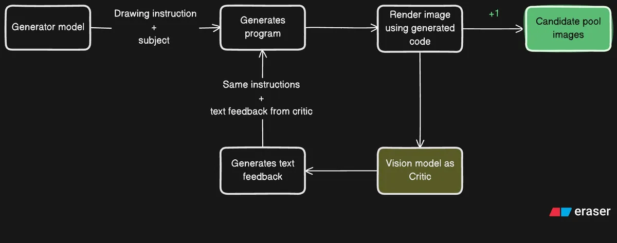
These 4 models which we call generators, received a fixed drawing instruction and a dynamic subject instruction of what to create to generate each candidate. The script cycles through the generator models and subjects to generate candidates. This is how the process looks like:

In order to generate a candidate, assign a generator model, a flower subject and a real photograph from iNaturalist dataset.
Generate first version of the image. The generator model receives the drawing instruction and subject as a prompt. It generates the code which is used to render the flower image.
Now it’s time for first feedback on this generated image. They pass the generated image to a vision model Qwen/Qwen3-VL-30B-A3B-Instruct along with the real photograph from iNaturalist that was assigned to this candidate in the beginning.
Vision model returns written visual feedback on color, petal structure, flower centre, foliage, and composition.
This feedback is appended to the earlier drawing instruction and subject prompt + the code generated by the generator model. It then makes another attempt and generate a second image.
We repeat the feedback process on this second image and the generator attempts again and generates the third image.
All 3 images that are generated i.e. the first attempt + 2 revisions are added to the candidate pool.
And this process goes on for the number of candidates attempt we want.

This entire process creates an exhaustive candidate pool of images from much capable models based on feedback using real world photographs.

Diagram showing a generator producing painting code, rendering candidate images, and revising the code using a vision critic’s feedback.

HF team vetted these images and labeled them Love or Okay based on how appealing the generated pictures were. This led to a final reference dataset of 178 images that will be used during training for evaluation and reward.

Reward function

We need a way to assess how the model is doing during RL, how to evaluate outputs and how to score them. This score later becomes a learning signal which helps us to update model weights to make better attempts more likely as training progresses.

Reward function starts with a validity check first. If the generated image doesn’t meet certain requirements, it gets 0 reward. Only after it passes the validity check, other scorers score the image.

Validity check	Reward $R$
Fails	$0$
Passes	$0.05 + 0.05 L + 0.60 J + 0.30 H$

Reward function is a weighted sum where $L$ is the length score, $J$ is the pairwise judge score, and $H$ is the quality score judged using a trained human preference model which takes an image and a description and outputs a score. Note that this is judge-led config of reward function. They actually ran 2 more training runs that were HPS led and HPS only. You can check the blog for more details.

Now let’s unpack each component of the reward function slightly.

Validity

This is just a deterministic code function which checks the generated image against a few conditions like it follows the required setup, uses a WEBGL canvas, has used p5.brush methods, has not loaded an external image and the canvas is not blank.

Once the image is generated, this check is run first. If rejected, the final reward is 0 for this image during the baseline evaluation and training.

Length

This rewards longer program to generate images. This is mainly to create differences between rollouts during the training and encourage more elaborate programs. However, length doesn’t guarantee that the model is getting better at generating flower paintings.

First, it estimates the number of tokens in the generated program which is used to render the image. This is just common heuristic.

t = \frac{number of characters in the code}{4}

Estimated token count $t$	Length score $L (t)$
$t < 150$	$0$
$150 \leq t < 3000$	$\frac{t - 150}{2850}$
$3000 \leq t \leq 6000$	$1$
$t > 6000$	$0$

For e.g. 1,575 estimated tokens would give $L = 0.5$ , contributing $0.5 \times 0.05 = 0.025$ to the total reward.

Pairwise judge

The role of this judge is to see how the generated image during training compares with images in the reference pool of 178 images which humans have vetted. However, we don’t compare the generated image with all 178 images. This is what it looks like:

The model generates an image during training.
Pick 4 images from the reference pool: 2 Love and 2 Okay. Each rollout in a training group is compared against these 4 references. We’re not picking 4 references each time for a rollout. This will become clear later in where we talk about how training loop works.
Make a pair of generated image with each of the 4 reference image. Show each pair in both orders i.e. in one, keep the reference image first and generated second. In another, vice versa. This would give total 8 comparison ways across 4 pairs for each generated image.
Pass this pair to a vision model which picks the better image A or B.
Score each reference comparison. If generated image wins both orders in a pair, it gets 1 as a score. If it only wins in 1 order it gets 0.5 and if losses in both it gets 0.
Average the 4 scores and this becomes the pairwise score for the generated painting.
Use this reward score with other components of the reward function.

Human preference score (HPS)

HPSv3 is a pre-trained vision language preference scorer. It receives the generated image and a fixed text description. The description is always “a loose watercolour flower” and it’s hardcoded. HPS then outputs a scalar which is converted into a score between 0 and 1. This is just a preference score that model has predicted. This doesn’t mean a painting is beautiful.

Reward shaping

We’ll see in a while how GRPO works, the RL algorithm they’ve used. But before that it’s important to understand why I think the reward function is designed the way it is.

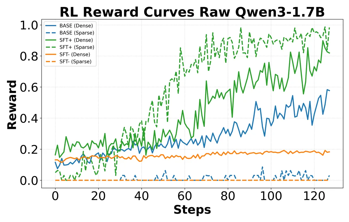
Even when every attempt fails the pairwise comparison, some of them would still be better in general and the reward should preserve that distinction so the model can get the learning signal.

This paper also talks about dense reward shaping and how it can help overcome an exploration bottleneck. During early training when complete success is too rare to sample, grading and rewarding partial success works. Rewarding partial success will reinforce the behavior and in turn would make complete success more likely to sample as training progresses.

Even if pairwise judge gives 0, HPS and Length can give different rewards across eligible rollouts. Now the differences in rewards can create non zero advantages and provide learning signal. If every rollout produces similar reward, the advantage is 0 and there’s nothing for the model to learn.

RL reward curves for Qwen3-1.7B comparing dense and sparse rewards for BASE, SFT+, and SFT- runs.

Rewards to learning signals

This is where everything comes together. Here we’ll see how the training loop works and how rewards are turned into learning signals for the model.

Algorithm used here is Group Relative Policy Optimization (GRPO). Simply put, in GRPO you generate multiple rollouts (or responses) from the current model (or policy). This is called a group or a training group. Each rollout in the group gets a reward based on the reward function. After that, you calculate the group reward mean. Now, you calculate advantage of each rollout within the group by subtracting the group mean and scale by standard deviation of group rewards.

Here, the number of rollouts per training group was selected as 8. Also, HF team disabled the scaling by standard deviation. You can explore why they did this. It’s a good learning exercise.

The model being trained is Qwen3.5-35B-A3B and they use LoRA.

Now, let’s go through one training loop step by step:

Step 1: Set the prompt

Start with the current policy and fixed prompt which has drawing instructions and subject instruction as Paint a peach hibiscus in loose watercolour.

Step 2: Sample eight responses

Sample eight responses from the current trainable policy using same prompt.

Step 3: Render and score each response

Render each image generated by the code, score them based on our reward function as explained earlier. Each rollout will get its own reward.

R_{i} = 0.05 + 0.05 L_{i} + 0.60 J_{i} + 0.30 H_{i}

Step 4: Calculate the group’s average reward

Calculate group’s average reward. Assume these are the rewards that each rollout got. We then average it.

R = [0, 0.3, 0.4, 0.5, 0.6, 0.7, 0.7, 0.8]

\bar{R} = \frac{4}{8} = 0.5

Step 5: Calculate each rollout’s advantage

Now calculate advantage for each rollout. For that subtract each rollout’s reward with group’s average reward. These numbers tell which sampled responses to encourage or discourage relative to the group.

A_{i} = R_{i} - \bar{R}

A = [- 0.5, - 0.2, - 0.1, 0, + 0.1, + 0.2, + 0.2, + 0.3]

Step 6: Run the sampled responses through the model

Run the above sampled responses through the model again to calculate gradients. For context, LLMs are autoregressive models. They generate one token at a time. So one response is made up to hundreds of tokens and LLM outputs the probability of the next token based on the context or prefix so far. So, during this step, we’re not sampling the response again as we’ve already done it to calculate rewards and advantages. We’re passing the already sampled responses to the policy and at each position it assigns the probability to the token that was generated.

Step 7: Calculate the GRPO loss

GRPO loss combines the token probabilities with the response’s advantage. Responses with positive advantage are pushed toward increasing the probability of sampled tokens in their context. Responses with negative advantage are pushed toward decreasing the probability of sampled tokens and responses with zero advantage contribute nothing.

Step 8: Update the model weights

The trainer calculates gradient of each rollout in a group at a time, accumulates gradients across 8 rollouts and then make 1 weights update.

Step 9: Repeat with the updated policy

Now repeat the same process with the new updated policy.

Bringing it all together

I still remember, when Surya’s tweet came out I tried recreating this but failed spectacularly. One thing stood out to me is choosing what to reward is part of defining what the model learns.

A higher reward in itself doesn’t mean the paintings that are generated are getting better. It’s just that model has learnt to game the reward system, if poorly designed. So next time, clearly define what does good look like, how we can measure it, do a baseline evaluation, train and see if the improvement is what we wanted.